A Peek into Deep Reinforcement Learning - Part I

I guess many of you interested in the field of Machine Learning have heard about DeepMind creating a system defeating the best professional human player in the Game of Go, called AlphaGo. I personally have never played Go before, so at first I wasn't aware of its complexity. Two years later they presented AlphaGo's successor called AlphaZero, which learned from scratch to master not only Go but also Chess and Shogi and defeated AlphaGo 100-0 without the use of domain knowledge or any human data. In December 2020 they presented the next evolution of this algorithm, called MuZero, which was able to master Go, Chess, Shogi and nearly all Atari games without knowing the rules of the game or the dynamics of the environment. After reading all of this it got my hooked and I wanted to know more about the algorithms and theory behind this magic - Reinforcement Learning (RL). In fact RL is around for quite some time now but in the last couple of years it really took off. Despite the truly impressive results of DeepMind, however, after a short research I also quickly realized that there are still relatively few viable real-world applications of reinforcement learning. However, I hope that this will change in the near future. To be honest, I am most excited about the applications in the field of robotics (e.g. Solving Rubik's Cube with Robotic Hand, Robotic Motor Adaptation) and autonomous driving. This prompted me to learn more about the field of Deep Reinforcement Learning and share my learnings with you in this blogpost.

Introduction into Reinfocement Learning

Before we dive into the algorithms and all that cool stuff I want to start with a short introduction into the most essential concepts and the terminology of RL. After that I give an overview of the framework for modeling those kinds of problems, called Markov Decision Processes (MDP) and I will present you a way to categorize deep RL algorithms.

Concepts and Terminology

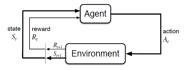
RL in general is concerned with solving sequential decision-making problems (e.g. playing video games, driving, robotic control, optimizing inventory) and such problems can be expressed as a system consisting of an agent which acts in an environment. These two are the core components of RL. The environment produces information which describes the state of the system and it can be considered to be anything that is not the agent. So, what is an agent then? An agent "lives" in and interacts with an environment by observing the state (or at least a part of it) and uses this information to select between actions to take. The environment accepts these actions and transitions into the next state and after that returns the next state and a reward to the agent. A reward signal is a single scalar the environment sents to the agent which defines the goal of the RL problem we want to solve. This whole cycle I have described so far is called one time-step and it repeats until/if the environment terminates (Figure 1.).

The action selection function the agent uses is called a policy, which maps states to actions. Every action will change the environment and affect what an agent observes and does next. To determine which actions to take in different situations every RL problems needs to have an objective or goal which is described by the sum of rewards received over time. The goal is to maximize the objective by selecting good actions which the agent learns by interacting with the environment in a process of trial-and-error combined with using the reward signals it receives to reinforce good actions. The exchange signal is often called experience and described as tuple of $(s_{t}, a_{t}, r_{t})$. Moreover we have to differentiate between finite and infinite environments. In finite environments $t=0,1,...,T$ is called one episode and a sequence of experiences over an episode $\tau = (s_{0}, a_{0}, r_{0}), (s_{1}, a_{1}, r_{1}), ...$ is called a trajectory. An agent typically needs many episodes to learn a good policy, ranging from hundreds to millions depending on the complexity of the problem. Now lets describe the states, actions and rewards a bit more formally:

• $s_{t} \in \mathcal{S}$ is the state, $\mathcal{S}$ is the state space
• $a_{t} \in \mathcal{A}$ is the action, $\mathcal{A}$ is the action space
• $r_{t} = \mathcal{R}(s_{t}, a_{t}, s_{t+1})$ is the reward, $\mathcal{R}$ is the reward function

Next we are diving into the framework for modeling those interactions between the agent and the environment called Markov Decision Processes.

RL as an Markov Decision Process

MDP in general is a mathematical framework for modeling sequential decision making and in RL the transitions of an environment between states is described as an MDP. The transition function has to meet the Markov property which assumes that the next state $s_{t+1}$ only depends on the previous state $s_{t}$ and action $a_{t}$ instead of the whole history of states and actions. When we talk about a state here it is also important to distinguish between the observed state $s_{t}$ from the agent and the environments internal state $s_{t}^{int}$ used by the transition function. In an MDP $s_{t} = s_{t}^{int}$ but in many interesting real-world problems the agent has only limited information and $s_{t} \neq s_{t}^{int}$. In those cases the environment is described as a partially oberservable MDP, in short POMDP.

All we need for the formal MDP description of a RL problem is a 4-tuple $\mathcal{S}$, $\mathcal{A}$, $P(.)$ and $\mathcal{R}(.)$:

• $\mathcal{S}$ is the set of states
• $\mathcal{A}$ is the set of actions
• $P(s_{t+1} \mid s_{t}, a_{t})$ is the state transition function of the environment
• $\mathcal{R}(s_{t}, a_{t}, s_{t+1})$ is the reward function of the environment

It is important to note that agents to have access to the transition function of the reward function, they only get information about these functions through the $(s_{t}, a_{t}, r_{t})$ tuples. The objective of an agent can be formalized by the return $R(\tau)$ using a trajectory from an episode

$$ R(\tau) = r_{0} + \gamma r_{1} + \gamma^{2} r_{2} + … + \gamma^{T} r_{T} = \sum_{t=0}^{T} \gamma^{t} r_{t} $$

$\gamma$ describes a discount factor which changes the way future rewards are valued. The objective $J(\tau)$ is simply the expectation of the returns over many trajectories

$$ J(\tau) = \mathbb{E}_{\tau \sim \pi} \big[R(\tau)\big] = \mathbb{E}_{\tau} \Big[\sum_{t=0}^{T} \gamma^{t} r_{t} \Big] $$

For problems with infinite time horizons it is important to set $\gamma < 1$ to prevent the objective from becoming unbounded.

Learnable Functions in RL

In RL there exist three primary functions which can be learned. One of them is the policy $\pi$ which maps states to actions: $a \sim \pi(s)$. This policy can be either deterministic or stochastic.

The second one is called a value function, $V^{\pi}$ or $Q^{\pi}(s,a)$, which estimates the expected return $\mathbb{E}_{\tau}[R(\tau)]$. Value functions provide information about the objective and thereby help an agent to understand how good the states and available actions are in terms of future rewards. As mentioned before, there exist two different versions of value functions:

$$ V^{\pi}(s) = \mathbb{E}_{s_{0} = s, \tau \sim \pi} \Big[\sum_{t=0}^{T} \gamma^{t} r_{t}\Big] $$

$$ Q^{\pi}(s,a) = \mathbb{E}_{s_{0} = s, a_{0} = a, \tau \sim \pi} \Big[\sum_{t=0}^{T} \gamma^{t} r_{t}\Big] $$

$V^{\pi}$ evaluates how good or bad a state is, assuming we continue with the current policy. $Q^{\pi}$ instead evaluates how good an action-state pair is.

The last of the three functions is the environment model or the transition function $P(s' \mid s,a)$ which provides information about the environment itself. If an agent learns this function, it is able to predict the next state $s'$ that the environment will transition into after taking action $a$ in state $s$. This gives the agent some kind of "imagination" about the consequences of its actions without interacting with the environment (planning).

All of the three functions discussed above can be learned so we can use deep neural networks as the function approximation method. Based on this you are also able to categorize deep RL algorithms.

Algorithms Overview

We can group RL algorithms based on the functions they learn into four different categories:

• Policy-based algorithms
• Value-based algorithms
• Model-based algorithms
• Combined Methods

Policy-based or policy optimization algorithms are a very general class of optimization methods which can be applied to problems with any type of actions, discrete, continuous or a mixture (multiaction). Moreover they are guaranteed to converge. The main drawbacks of these algorithms are that they have a high variance and are sample inefficient.

Most of the value-based algorithms learn $Q^{\pi}$ instead of $V^{\pi}$ because it is easier to convert into a policy. Moreover they are typically more sample efficient than policy-based algorithms because they have lower variance and make better use of data gathered from the environment. But they don't have a convergence guarantee and are only applicable to discrete action spaces (*QT-OPT* can also be applied to continuous action spaces).

As mentioned before model-based algorithms learn a model of the environments transition dynamics or make use of a known dynamics model. The agent can use this model to "imagine" what will happen in the future by predicting the trajectory for a few time steps. Purely model-based approaches are commonly applied to games with a target state or navigation tasks with a goal state. These kinds of algorithms are very appealing because they equip an agent with foresight and need a lot fewer samples of data to learn good policies. But for most problems, models are hard to come by because many environments are stochastic, their transition dynamics are not known and the model therefore must be learned (which is pretty hard in large state spaces).

These days many combined methods try to get the best of each, e.g. Actor-Critic algorithms learn a policy and a value function where the policy acts and the value function critiques those actions. Another popular example would be AlphaZero which combined Monte Carlo Tree Search with learning $V^{\pi}$ and a policy $\pi$ to master the game of Go.

In Figure 2 you can see a slightly different way of categorizing these algorithms, by first differentiating between model-based and model-free methods.

Another possibility to distinguish between these algorithms would be:

• on-policy: Training can only utilize data generated from the current policy $\pi$ which tends to be sample-inefficient and needs more training data.
• off-policy: Any data collected can be reused in training which is more sample-efficient but requires much more memory.

In the following we are going to describe three different algorithms. One of them is a policy-based algorithm called REINFORCE (Policy Gradient). The other two are value-based algorithms called SARSA and Deep Q-Networks. In the second part of this post I will also go into some more advanced combined methods.

Policy Gradient - REINFORCE

The REINFORCE algorithm was invented in 1992 by Ronald J. Williams. It learns a parameterized policy which produces action probabilities from states and an agent can use this policy directly to act in an environment. The action probabilities are changed by following the policy gradient. The algorithm has three core components:

• parameterized policy
• objective to be maximized
• method for updating the policy parameters

A neural network is used to learn a good policy by function approximation. This is often called a policy network $\pi_{\theta}$ (parameterized by $\theta$). The objective function to maximize is the expected return over all complete trajectories generated by an agent:

$$ J(\pi_{\theta}) = \mathbb{E}_{\tau \sim \pi_{\theta}} \big[ R(\tau) \big] = \mathbb{E}_{\tau \sim \pi_{\theta}} \Big[ \sum_{t=0}^{T} \gamma^{t} r_{t} \Big] $$

To maximize this objective, gradient ascent is performed on the policy parameters $\theta$. The parameters are then updated based on:

$$ \theta \leftarrow \theta + \alpha \nabla_{\theta} J(\pi_{\theta}) $$

The term $\nabla_{\theta} J(\pi_{\theta})$ is known as the policy gradient and is defined as:

$$ \nabla_{\theta} J(\pi_{\theta}) = \mathbb{E}_{\tau \sim \pi_{\theta}} \Big[ \sum_{t=0}^{T} R_{t}(\tau) \nabla_{\theta} \log \pi_{\theta} (a_{t} | s_{t})\Big] $$

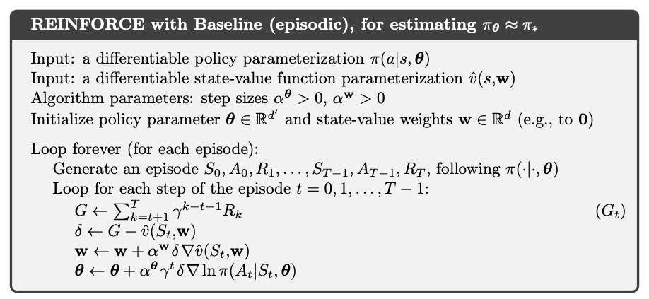
The policy gradient is numerically estimated using Monte Carlo Sampling which refers to any method that uses random sampling to generate data used to approximate a function. Now lets take a look at the pseudocode for the algorithm:

One problem of REINFORCE is the policy gradient estimate can have high variance. One way to reduce this is by introducing a baseline (see Figure 3). Next we are going to learn about two popular value-based algorithms, SARSA and Q-Networks. If you are interested in how the actual code would look like, check out my RL repository.

SARSA

SARSA (State-action-reward-state-action) is a value-based on-policy method which aims to learn the Q-function $Q^{\pi}(s,a)$. It is based on two core ideas:

1. Temporal Difference Learning for learning the Q-function
2. Generate actions using the Q-function

In Temporal Difference Learning (TD-Learning) a neural network is used to produce Q-value estimates given $(s,a)$ pairs as input. This is called value network. The general learning workflow is pretty similar to a classical supervised learning workflow:

1. Generate trajectories $\tau$s and predict a $\hat{Q}$-value for each $(s,a)$-pair
2. Generate target Q-values $Q_{tar}$ based on the trajectories.
3. Minimize the distance between $\hat{Q}$ and $Q_{tar}$ using a standard regression loss (like MSE)
4. Repeat 1-3

If we would want to use Monto Carlo Sampling here, an agent would have to wait for episodes to end before any data from that episode can be used to learn from, which delays training. We can use TD-Learning to circumvent this problem. The key insight here is that we can define Q-values for the current time step in terms of Q-values of the next time step. This recursive definition is known as the Bellman Equation:

$$ Q^{\pi}(s,a) \approx r + \gamma Q^{\pi}(s’,a’) = Q^{\pi}_{tar}(s,a) $$

But if we use the same policy to generate $\hat{Q}^{\pi}(s,a)$ and $Q_{tar}^{\pi}(s,a)$ but how does this work or learn at all? This is possible because $Q_{tar}^{\pi}(s,a)$ uses information one time step into the future when compared with $\hat{Q}^{\pi}(s,a)$. Thus it has access to the reward $r$ from the next state $s'$ ($Q_{tar}^{\pi}(s,a)$ is slightly more informative about how the trajectory will turn out). TD Learning gives us a method for learning how to evaluate state action pairs, but what about choosing the actions?

If we already learned the optimal Q-function, the value of each state-action pair will represent the best possible expected value from taking that action, so we can act greedily with respect to those Q-values. The problem is that this optimal Q-function isn't typically known in advance. But we can use an iterative approach to improve the Q-value by improving the Q-function:

1. Initialize a neural network randomly with the parameters $\theta$ to represent the Q-function $Q^{\pi}(s,a;\theta)$
2. Repeat the following until the agent stops improving:
   1. Use $Q^{\pi}(s,a;\theta)$ to act in the environment, by action greedily (or $\varepsilon$-greedy) with respect to the Q-values and store all of the experiences $(s,a,r,s’)$.
   2. Use the stored experiences to update $Q^{\pi}(s,a;\theta)$ using the Bellman equation to improve the Q-function estimate, which, in turn, improves the policy.

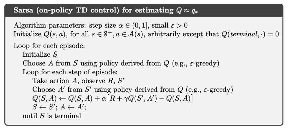
A greedy action selection policy is deterministic and might lead to an agent not exploring the whole state-action space. To mitigate this issue a so called $\varepsilon$-greedy policy is often used in practice, where you act greedy with probability 1-$\varepsilon$ and random with probability $\varepsilon$. A common strategy here is to start training with a high $\varepsilon$ (e.g. 1.0) so that the agent almost acts randomly and rapidly explores the state-action space. Decay $\varepsilon$ gradually over time so that after many steps the policy, hopefully, approaches the optimal policy. The figure down below shows the pseudocode for the whole SARSA algorithm.

In the next section we are going to learn more about another popular value-based method called Deep Q-Networks.

Deep Q-Networks

General Concept

Deep Q-Networks (DQN) were proposed by Mnih et al. in 2013 and are like SARSA a value-based temporal difference learning algorithm that approximates the Q-function. It is also only applicable to environments with discrete action spaces. Instead of learning the Q-function for the current policy DQN learns the optimal Q-function which improves its stability and learning speed over SARSA. This makes it an off-policy algorithm because the optimal Q-function does not depend on the data gathering policy. This also makes it more sample efficient than SARSA. The main difference between the two is the $Q^{\pi}_{tar}(s,a)$ construction:

$$ Q^{\pi}_{tar}(s,a) = r + \gamma \max_{a’} Q^{\pi}(s’,a’) $$

Instead of using the action $a'$ actually taken in the next state $s'$ to estimate $Q^{\pi}_{tar}(s,a)$, DQN uses the maximum Q-value over all of the potential actions available in that state, which makes it independent from the policy. For action selection you can use e.g. $\epsilon$-greedy or Boltzmann policy. The $\epsilon$-greedy exploration strategy is somewhat naive because the exploration is random and do not use any previously learned knowledge about the environment. In contrast the Boltzmann policy tries to improve on this by selecting actions based on their relative Q-values which has the effect of focusing exploration on more promising actions. It is a parameterized softmax function, where a temperature parameter $\tau \in (0, \infty)$ controls how uniform or concentrated the resulting probability distribution is:

$$ p(a|s) = \frac{e^{Q^{\pi}(s,a)/\tau}}{\sum_{a’}e^{Q^{\pi}(s,a’)/\tau}} $$

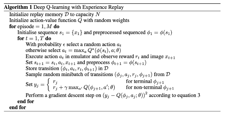
The role of the temperature parameter $\tau$ in the Boltzmann policy is analoguous to that of $\epsilon$ in the $\epsilon$-greedy policy. It encourages exploration of the state-action space, a high value for $\tau$ means more exploration. To balance exploration and exploitation during training, $\tau$ is adjusted properly (decreased over time). The Boltzmann policy is often more stable than the $\epsilon$-greedy policy but it also can cause an agent to get stuck in a local minimum if the Q-function estimate is inaccurate for some parts of the state space. This can be tackled by using a very large value for $\tau$ at the beginning of training. As mentioned at the beginning of this section, DQN is an off-policy algorithm that doesn't have to discard experiences once they have been used, so we need a so called experience-replay memory to store these experiences for the training. It stores the $k$ most recent experiences an agent has gathered and if the memory is full, older experiences will be discarded. The size of the memory should be large enough to contain many episodes of experiences, so that each batch will contain experiences from different episodes and policies. This will decorrelate the experiences used for training and reduce the variance of the parameter updates, helping to stabilize training. Down below you can the full algorithm from the paper.

DQN Improvements

Over time people have explored multiple ways to improve the DQN algorithm which we will talk about in the last part of this post. The three modifications are the following:

1. Target networks
2. Double DQN
3. Prioritized Experience Replay

Target Networks

In the original DQN algorithm $Q_{tar}^{\pi}$ is constantly changing because it depends on $\hat{Q}^{\pi}(s,a)$. This makes it kind of a "moving target" which can destabilize training because it makes it unclear what the network should learn. To reduce the changes in $Q_{tar}^{\pi}(s,a)$ between training steps, you can use a target network. Second network with parameters $\varphi$ which is a lagged copy of the Q-network $Q^{\pi_{\theta}}(s,a)$. It gets periodically updated to the current values for $\theta$, which is called a replacement update. The update frequency is problem dependent (1000 - 10000, for complex environments and 100 - 1000 for simpler ones). Down below you can see the modified Bellman equation:

$$ Q_{tar}^{\pi_{\varphi}}(s,a) = r + \gamma \max_{a’}Q^{\pi_{\varphi}}(s’,a’) $$

Introducing this network stops the target from moving and transforms the problem into a standard supervised regression. An alternative to the periodic replacement is the so called Polyak update. At each time step, set $\varphi$ to be a weighted average of $\varphi$ and $\theta$, which makes $\varphi$ change more slowly than $\theta$. The hyperparameter $\beta$ controls the speed at which $\varphi$ changes:

$$ \varphi \leftarrow \beta \varphi + (1 - \beta) \theta $$

It is important to note that each approach has its advantages and disadvantages and no one is clearly better than the other.

Double DQN

The Double DQN addresses the problem of overestimating Q-values. If you want to know in detail about why this actually happens, take a look at the following paper. The Q-value overestimation can hurt exploration and the error it causes will be backpropagated in time to earlier (s,a)-pairs which adds error to those as well. Double DQN reduces this by learning two Q-function estimates using different experiences. The Q-maximizing action $a'$ is selected using the first estimate and the Q-value that is used to calculate $Q_{tar}^{\pi}(s,a)$ is generated by the second estimate using the before selected action. This removes the bias and leads to the following:

$$ Q_{tar: DDQN}^{\pi}(s,a) = r + \gamma Q^{\pi_{\varphi}} \big(s’, \max_{a’}Q^{\pi_{\theta}}(s’,a’) \big) $$

If the number of time steps between the target network and the training network is large enough, we could use this one for the Double DQN.

Prioritized Experience Replay

The main idea behind this is that some experiences in the replay memory are more informative than others. So if we can train an agent by sampling informative experiences more often then the agent may learn faster. To achieve this, we have to answer the following two questions:

1. How can we automatically assign a priority to each experience?
2. How to sample efficiently from the replay memory using these priorities?

As the priority we can simply use the TD error without much computational overhead. At the start of training the priorities of all values are set to a large constant value to encourage each experience to be sampled at least once. The sampling could be done rank-based or based on proportional prioritization. For details on the rank based prioritization, take a look at this paper. The priority for the proportional method is calculated as follows:

$$ P(i) = \frac{(|\omega_{i}| + \epsilon)^{\eta}}{\sum_{j}(|\omega_{i}| + \epsilon)^{\eta}} $$

where $\omega_{i}$ is the TD error of experience $i$, $\epsilon$ is a small positive number and $\eta$. $\eta$ determines how much to prioritize, so that the larger the $\eta$ the greater the prioritization. Prioritizing certain examples changes the expectation of the entire data distribution, which introduces bias into the training process. This can be corrected by multiplying the TD error for each example by a set of weights, which is called importance sampling.

Summary

In this post I have tried to give a very short intro to the basic terminology of Reinforcement Learning. If you are interested in this field I encourage you to take a look a Barto and Suttons Reinforcement Learning: An Introduction) and the great resource OpenAI Spinning Up created by Josh Achiam.

Moreover we've seen a way to categorize the different algorithm families of RL. I summarized one policy gradient algorithm called REINFORCE (there exist way more out there) for you to give you a better understanding of the concept of policy learning. After that we explored two value-based algorithms in SARSA and DQN, and we looked at a few tricks to further improve the performce of DQN. In the next part of this series of posts, I'm going to dive deeper in a few more modern deep RL algorithms and combined methods we talked about.

References

[1] Barto and Sutton, Reinforcement Learning: An Introduction (2018).

[2] Josh Achiam, OpenAI Spinning Up (2018).

[3] Mnih et al., Playing Atari with Deep Reinforcement Learning (2013).

[4] van Hasselt et al., Deep Reinforcement Learning with Double Q-Learning (2015).

[5] Graesser and Keng, Foundations of Deep Reinforcement Learning (2019).

[6] Schaul et al., Prioritized Experience Replay (2016).